Interpreting Deep Neural Networks with SVCCA

Posted by Maithra Raghu, Google Brain Team

Deep neural networks (DNNs) have driven unprecedented advances in areas such as vision, language understanding and speech recognition. But these successes also bring new challenges. In particular, contrary to many previous machine learning methods, DNNs can be susceptible to adversarial examples in classification, catastrophic forgetting of tasks in reinforcement learning, and mode collapse in generative modelling. In order to build better and more robust DNN-based systems, it is critically important to be able to interpret these models. In particular, we would like a notion of representational similarity for DNNs: can we effectively determine when the representations learned by two neural networks are same?

In our paper, “SVCCA: Singular Vector Canonical Correlation Analysis for Deep Learning Dynamics and Interpretability,” we introduce a simple and scalable method to address these points. Two specific applications of this that we look at are comparing the representations learned by different networks, and interpreting representations learned by hidden layers in DNNs. Furthermore, we are open sourcing the code so that the research community can experiment with this method.

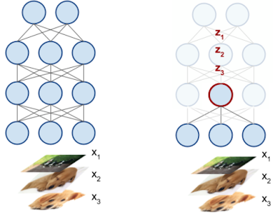
Key to our setup is the interpretation of each neuron in a DNN as an activation vector. As shown in the figure below, the activation vector of a neuron is the scalar output it produces on the input data. For example, for 50 input images, a neuron in a DNN will output 50 scalar values, encoding how much it responds to each input. These 50 scalar values then make up an activation vector for the neuron. (Of course, in practice, we take many more than 50 inputs.)

Here a DNN is given three inputs, x1, x2, x3. Looking at a neuron inside the DNN (bolded in red, right pane), this neuron produces a scalar output zi corresponding to each input xi. These values form the activation vector of the neuron.

With this basic observation and a little more formulation, we introduce Singular Vector Canonical Correlation Analysis (SVCCA), a technique for taking in two sets of neurons and outputting aligned feature maps learned by both of them. Critically, this technique accounts for superficial differences such as permutations in neuron orderings (crucial for comparing different networks), and can detect similarities where other, more straightforward comparisons fail.

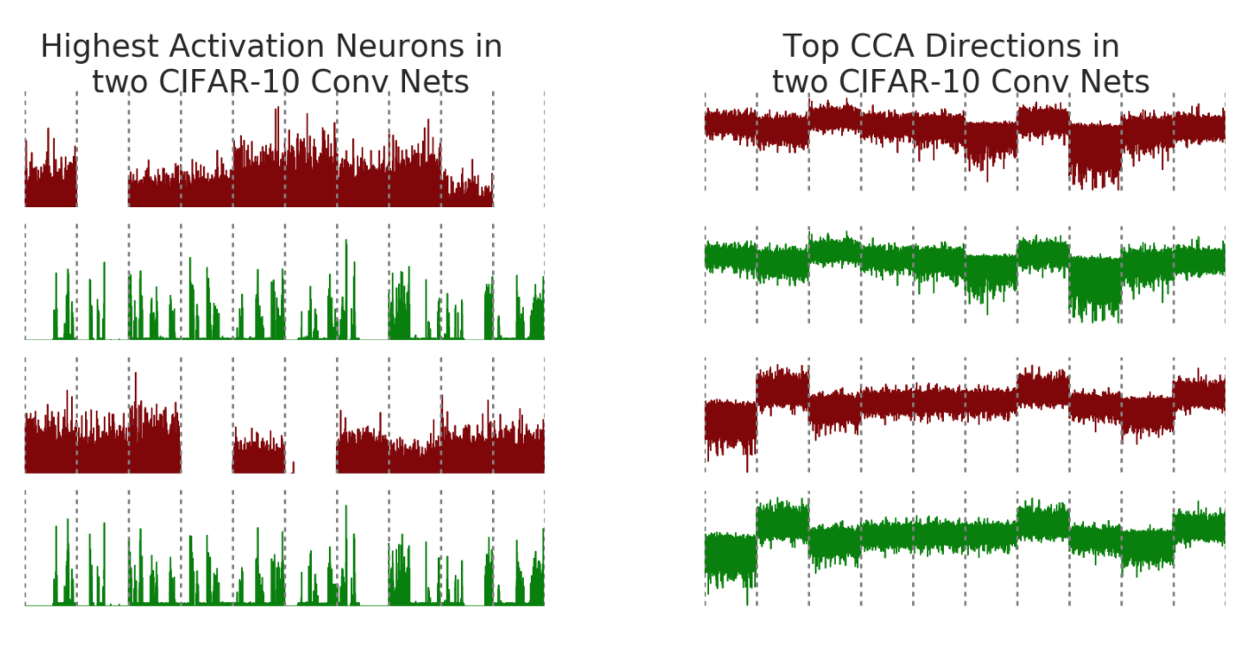
As an example, consider training two convolutional neural nets (net1 and net2, below) on CIFAR-10, a medium scale image classification task. To visualize the results of our method, we compare activation vectors of neurons with the aligned features output by SVCCA. Recall that the activation vector of a neuron is the raw scalar outputs on input images. The x-axis of the plot consists of images sorted by class (gray dotted lines showing class boundaries), and the y axis the output value of the neuron.
On the left pane, we show the two highest activation (largest euclidean norm) neurons in net1 and net2. Examining highest activations neurons has been a popular method to interpret DNNs in computer vision, but in this case, the highest activation neurons in net1 and net2 have no clear correspondence, despite both being trained on the same task. However, after applying SVCCA, (right pane), we see that the latent representations learned by both networks do indeed share some very similar features. Note that the top two rows representing aligned feature maps are close to identical, as are the second highest aligned feature maps (bottom two rows). Furthermore, these aligned mappings in the right pane also show a clear correspondence with the class boundaries, e.g. we see the top pair give negative outputs for Class 8, with the bottom pair giving a positive output for Class 2 and Class 7.

While you can apply SVCCA across networks, one can also do this for the same network, across time, enabling the study of how different layers in a network converge to their final representations. Below, we show panes that compare the representation of layers in net1 during training (y-axes) with the layers at the end of training (x-axes). For example, in the top left pane (titled “0% trained”), the x-axis shows layers of increasing depth of net1 at 100% trained, and the y axis shows layers of increasing depth at 0% trained. Each (i,j) square then tells us how similar the representation of layer i at 100% trained is to layer j at 0% trained. The input layer is at the bottom left, and is (as expected) identical at 0% to 100%. We make this comparison at several points through training, at 0%, 35%, 75% and 100%, for convolutional (top row) and residual (bottom row) nets on CIFAR-10.

Plots showing learning dynamics of convolutional and residual networks on CIFAR-10. Note the additional structure also visible: the 2x2 blocks in the top row are due to batch norm layers, and the checkered pattern in the bottom row due to residual connections.

We find evidence of bottom-up convergence, with layers closer to the input converging first, and layers higher up taking longer to converge. This suggests a faster training method, Freeze Training — see our paper for details. Furthermore, this visualization also helps highlight properties of the network. In the top row, there are a couple of 2x2 blocks. These correspond to batch normalization layers, which are representationally identical to their previous layers. On the bottom row, towards the end of training, we can see a checkerboard like pattern appear, which is due to the residual connections of the network having greater similarity to previous layers.

So far, we’ve concentrated on applying SVCCA to CIFAR-10. But applying preprocessing techniques with the Discrete Fourier transform, we can scale this method to Imagenet sized models. We applied this technique to the Imagenet Resnet, comparing the similarity of latent representations to representations corresponding to different classes:

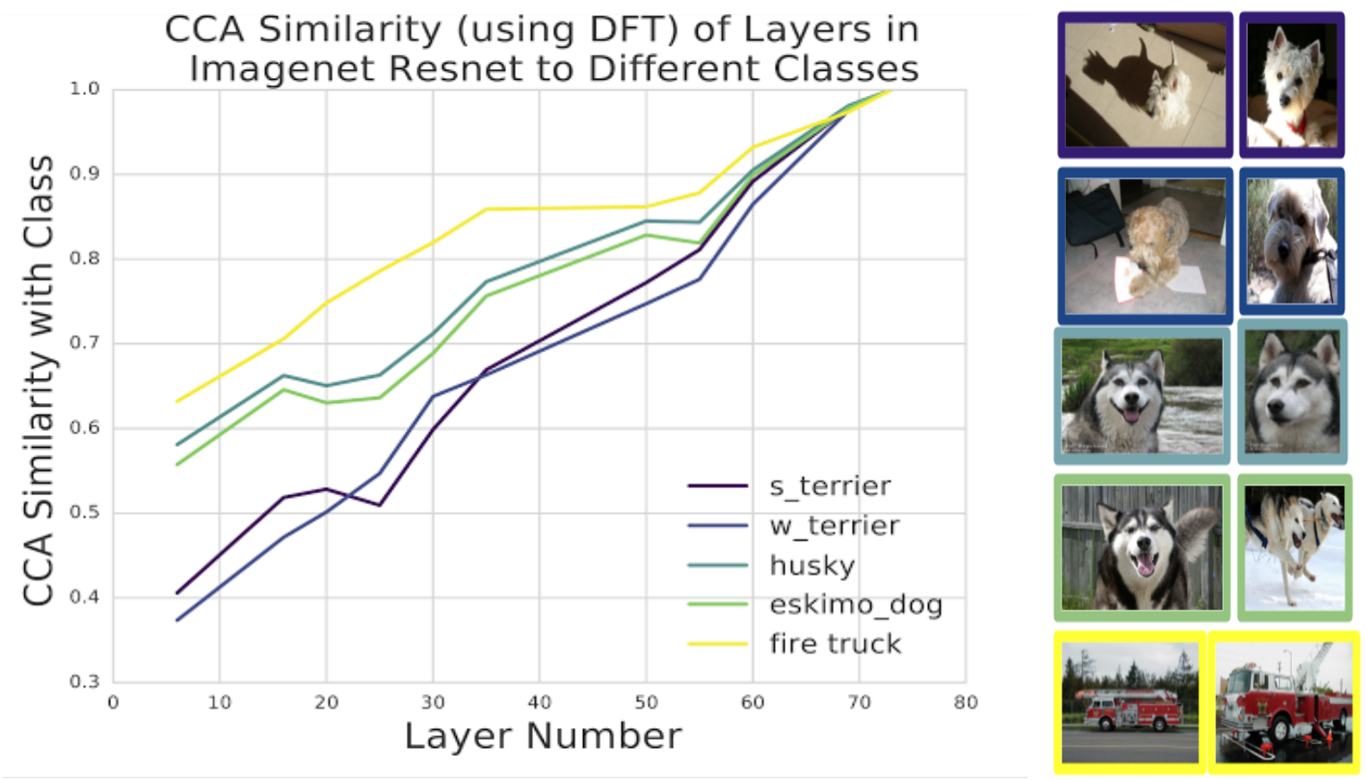SVCCA similarity of latent representations with different classes. We take different layers in Imagenet Resnet, with 0 indicating input and 74 indicating output, and compare representational similarity of the hidden layer and the output class. Interestingly, different classes are learned at different speeds: the firetruck class is learned faster than the different dog breeds. Furthermore, the two pairs of dog breeds (a husky-like pair and a terrier-like pair) are learned at the same rate, reflecting the visual similarity between them.

Our paper gives further details on the results we’ve explored so far, and also touches on different applications, e.g. compressing DNNs by projecting onto the SVCCA outputs, and Freeze Training, a computationally cheaper method for training deep networks. There are many followups we’re excited about exploring with SVCCA — moving on to different kinds of architectures, comparing across datasets, and better visualizing the aligned directions are just a few ideas we’re eager to try out. We look forward to presenting these results next week at NIPS 2017 in Long Beach, and we hope the code will also encourage many people to apply SVCCA to their network representations to interpret and understand what their network is learning.