
Using Machine Learning to “Nowcast” Precipitation in High Resolution
January 13, 2020
Posted by Jason Hickey, Senior Software Engineer, Google Research
The weather can affect a person’s daily routine in both mundane and serious ways, and the precision of forecasting can strongly influence how they deal with it. Weather predictions can inform people about whether they should take a different route to work, if they should reschedule the picnic planned for the weekend, or even if they need to evacuate their homes due to an approaching storm. But making accurate weather predictions can be particularly challenging for localized storms or events that evolve on hourly timescales, such as thunderstorms.
In “Machine Learning for Precipitation Nowcasting from Radar Images,” we are presenting new research into the development of machine learning models for precipitation forecasting that addresses this challenge by making highly localized “physics-free” predictions that apply to the immediate future. A significant advantage of machine learning is that inference is computationally cheap given an already-trained model, allowing forecasts that are nearly instantaneous and in the native high resolution of the input data. This precipitation nowcasting, which focuses on 0-6 hour forecasts, can generate forecasts that have a 1km resolution with a total latency of just 5-10 minutes, including data collection delays, outperforming traditional models, even at these early stages of development.
Moving Beyond Traditional Weather Forecasting
Weather agencies around the world have extensive monitoring facilities. For example, Doppler radar measures precipitation in real-time, weather satellites provide multispectral imaging, ground stations measure wind and precipitation directly, etc. The figure below, which compares false-color composite radar imaging of precipitation over the continental US to cloud cover imaged by geosynchronous satellites, illustrates the need for multi-source weather information. The existence of rain is related to, but not perfectly correlated with, the existence of clouds, so inferring precipitation from satellite images alone is challenging.
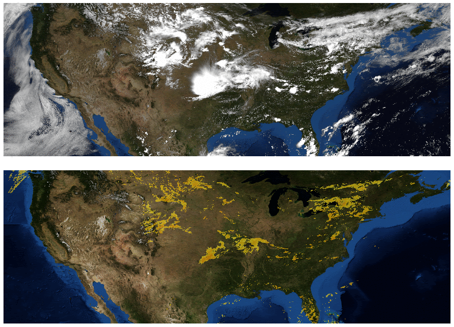 |
| Top: Image showing the location of clouds as measured by geosynchronous satellites. Bottom: Radar image showing the location of rain as measured by Doppler radar stations. (Credit: NOAA, NWS, NSSL) |
Even so, there is so much observational data in so many different varieties that forecasting systems struggle to incorporate it all. In the US, remote sensing data collected by the National Oceanic and Atmospheric Administration (NOAA) is now reaching 100 terabytes per day. NOAA uses this data to feed the massive weather forecasting engines that run on supercomputers to provide 1- to 10-day global forecasts. These engines have been developed over the course of the last half century, and are based on numerical methods that directly simulate physical processes, including atmospheric dynamics and numerous effects like thermal radiation, vegetation, lake and ocean effects, and more.
However, the availability of computational resources limits the power of numerical weather prediction in several ways. For example, computational demands limit the spatial resolution to about 5 kilometers, which is not sufficient for resolving weather patterns within urban areas and agricultural land. Numerical methods also take multiple hours to run. If it takes 6 hours to compute a forecast, that allows only 3-4 runs per day and resulting in forecasts based on 6+ hour old data, which limits our knowledge of what is happening right now. By contrast, nowcasting is especially useful for immediate decisions from traffic routing and logistics to evacuation planning.
Radar-to-Radar Forecasting
As a typical example of the type of predictions our system can generate, consider the radar-to-radar forecasting problem: given a sequence of radar images for the past hour, predict what the radar image will be N hours from now, where N typically ranges from 0-6 hours. Since radar data is organized into images, we can pose this prediction as a computer vision problem, inferring the meteorological evolution from the sequence of input images. At these short timescales, the evolution is dominated by two physical processes: advection for the cloud motion, and convection for cloud formation, both of which are significantly affected by local terrain and geography.
 |
| Top (left to right): The first three panels show radar images from 60 minutes, 30 minutes, and 0 minutes before now, the point at which a prediction is desired. The right-most panel shows the radar image 60 minutes after now, i.e., the ground truth for a nowcasting prediction. Bottom Left: For comparison, a vector field induced from applying an optical flow (OF) algorithm for modeling advection to the data from the first three panels above. Optical flow is a computer vision method that was developed in the 1940s, and is frequently used to predict short term weather evolution. Bottom Right: An example prediction made by OF. Notice that it tracks the motion of the precipitation in the bottom left corner well, but fails to account for the decaying strength of the storm. |
CNNs are usually composed of a linear sequence of layers, where each layer is a set of operations that transform some input image into a new output image. Often, a layer will change the number of channels and the overall resolution of the image it’s given, in addition to convolving the image with a set of convolutional filters. These filters are themselves small images (for us, they are typically only 3x3, or 5x5). Filters drive much of the power of CNNs, and result in operations like detecting edges, identifying meaningful patterns, etc.
A particularly effective type of CNN is the U-Net. U-Nets have a sequence of layers that are arranged in an encoding phase, in which layers iteratively decrease the resolution of the images passing through them, and then a decoding phase in which the low-dimensional representations of the image created by the encoding phase are expanded back to higher resolutions. The following figure shows all of the layers in our particular U-Net.
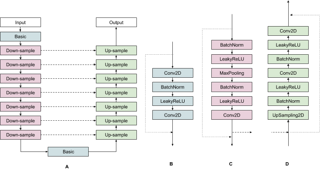 |
| (A) The overall structure of our U-NET. Blue boxes correspond to basic CNN layers. Pink boxes correspond to down-sample layers. Green boxes correspond to up-sample layers. Solid lines indicate input connections between layers. Dashed lines indicate long skip connections transversing the encoding and decoding phases of the U-NET. Dotted lines indicate short skip connections for individual layers. (B) The operations within our basic layer. (C) The operations within our down-sample layers. (D) The operations within our up-sample layers. |
Results
We compare our results with three widely used models. First, the High Resolution Rapid Refresh (HRRR) numerical forecast from NOAA. HRRR actually contains predictions for many different weather quantities. We compared our results to their 1-hour total accumulated surface precipitation prediction, as that was their highest quality 1-hour precipitation prediction. Second, an optical flow (OF) algorithm, which attempts to track moving objects through a sequence of images. This latter approach is often applied to weather prediction even though it makes the assumption that overall rain quantities over large areas are constant over the prediction time — an assumption that is clearly violated. Third, the so-called persistence model, is the trivial model in which each location is assumed to be raining in the future at the same rate it is raining now, i.e. the precipitation pattern does not change. That may seem like an overly simplistic model to compare to, but it is common practice given the difficulty of weather prediction.
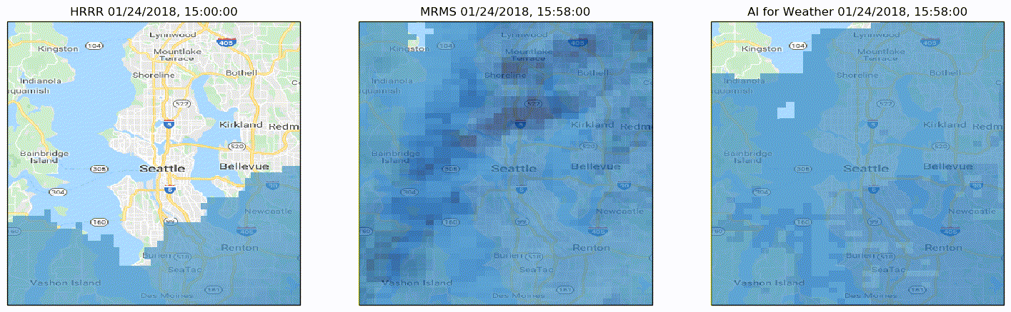 |
| A visualization of predictions made over the course of roughly one day. Left: The 1-hour HRRR prediction made at the top of each hour, the limit to how often HRRR provides predictions. Center: The ground truth, i.e., what we are trying to predict. Right: The predictions made by our model. Our predictions are every 2 minutes (displayed here every 15 minutes) at roughly 10 times the spatial resolution made by HRRR. Notice that we capture the general motion and general shape of the storm. |
 |
| Precision and recall (PR) curves comparing our results (solid blue line) with: optical flow (OF), the persistence model, and the HRRR 1-hour prediction. As we do not have direct access to their classifiers, we cannot provide a full PR curve for their results. Left: Predictions for light rain. Right: Predictions for moderate rain. |
Acknowledgements
Thanks to Carla Bromberg, Shreya Agrawal, Cenk Gazen, John Burge, Luke Barrington, Aaron Bell, Anand Babu, Stephan Hoyer, Lak Lakshmanan, Brian Williams, Casper Sønderby, Nal Kalchbrenner, Avital Oliver, Tim Salimans, Mostafa Dehghani, Jonathan Heek, Lasse Espeholt, Sella Nevo, Avinatan Hassidim.
Other posts of interest
-
April 23, 2024
Safely repairing broken builds with ML- Machine Intelligence ·
- Software Systems & Engineering
-

April 17, 2024
Robust speech recognition in AR through infinite virtual rooms with acoustic modeling- Human-Computer Interaction and Visualization ·
- Machine Perception ·
- Speech Processing
-
April 12, 2024
Contrastive neural audio separation- Machine Intelligence ·
- Sound & Accoustics